How to Use Lookup Function in Excel: A Step-by-Step Guide
How to Use Lookup Function in Excel is the single most important skill that separates a spreadsheet user from a data strategist. In my experience within the EdTech and industrial accounting sectors, I’ve realised that data is rarely in one place. It’s fragmented. Your student names are in one portal, their fee status is in another, and their exam results are in a third.
In the niche of industrial accounting, this fragmentation is even more severe. You have inventory codes in your ERP (like SAP or Oracle), tax rates in a government PDF, and manual adjustments in a Tally export. Without lookup functions, you are stuck in the manual copy-paste trap, a trap that leads to human error, missed deadlines, and GST filing disasters.
This guide isn’t just a tutorial; it’s a masterclass designed to make you the most indispensable person in your office. By the time you finish reading, you won’t just know the formulas, you’ll understand the logic of data architecture.
Table of Contents
- What Are Lookup Functions in Excel?
- Excel Lookup Functions List
- VLOOKUP: The Workhorse of the Industrial Age
- HLOOKUP: Mastering the Horizontal Grid
- XLOOKUP: The VLOOKUP Killer and Modern Standard
- INDEX & MATCH
- Beginner Example: Using VLOOKUP to Find Product Prices
- Common Lookup Errors in Excel and How to Fix Them
- Advanced Lookup Techniques
- Industry Use Case: SAP, Tally, and GST Reconciliation
- Performance Optimization: Handling 1,000,000 Rows
- Comparison Table: XLOOKUP vs VLOOKUP vs INDEX MATCH
- Conclusion
- Frequently Asked Questions
What Are Lookup Functions in Excel?
Lookup functions are specialized formulas designed to search for a specific value in one data range and return a corresponding piece of information from another. Their primary purpose is to automate the retrieval and cross-referencing of data between different tables, sheets, or workbooks.
Why are they used in data analysis?
- Relational Mapping: They connect two different datasets via a unique “Key” (like a GSTIN or Student ID).
- Audit Accuracy: They eliminate the 5% error rate typical of manual data entry.
- Dynamic Reporting: They allow dashboards to update automatically when source data changes.
- Scalability: They enable users to process 100,000+ rows of data in seconds.

Excel Lookup Functions List
To navigate the world of data retrieval, you must choose the right tool for the specific architectural challenge you face.
| Function Name | Purpose | Example Use Case |
|---|---|---|
| VLOOKUP | Searches vertically down the first column. | Matching a Tally Ledger name to an SAP Vendor Code. |
| HLOOKUP | Searches horizontally across the first row. | Pulling tax percentages from a horizontal GST slab. |
| XLOOKUP | Modern, flexible search in any direction. | The “Go-to” for 90% of modern accounting tasks. |
| INDEX MATCH | Two-step lookup for complex structures. | Large-scale inventory management (500k+ rows). |
| FILTER | Returns all matches as a dynamic list. | Listing all students who failed a specific subject. |
VLOOKUP: The Workhorse of the Industrial Age
The VLOOKUP function in Excel (Vertical Lookup) has been the industry standard since the 1980s. While modern alternatives exist, 90% of the corporate world still speaks the language of VLOOKUP. If you are sharing files with a client using an older version of Excel, this is your primary tool.
The Mechanics: How it Works
VLOOKUP searches for a value in the first column of a table and returns a value in the same row from a column you specify.
Excel =VLOOKUP(lookup_value, table_array, col_index_num, [range_lookup])
Step-by-Step VLOOKUP for SAP Data Reconciliation:
Imagine you have a list of SAP Document Numbers in Column A and you need to pull the Vendor Name from a Master List located on another sheet.
- Lookup Value: The Document Number (e.g., 45000123). This is your “anchor.”
- Table Array: The Master List range (e.g., ‘Master’!$A$2:$G$5000). Use F4 to lock this into an absolute reference.
- Column Index Number: Count from the left of your selection. If Vendor Name is the 3rd column, enter 3.
- Range Lookup: Always use FALSE (or 0) for an exact match.
The Left-Hand Limitation: A Professional Warning
VLOOKUP cannot look behind it. If your “Key” is in Column C, you cannot pull data from Column A or B. This is why many junior accountants spend hours moving columns around, a practice I strictly advise against because it breaks other linked sheets. Instead, use a “Helper Column” or upgrade to XLOOKUP or INDEX MATCH.

HLOOKUP: Mastering the Horizontal Grid
While we usually think of data in columns, the HLOOKUP function in Excel (Horizontal Lookup) is vital for specific accounting structures, such as depreciation schedules or tax slabs, where headers are listed horizontally.
When to use HLOOKUP in Excel with example:
Consider a GST Tax Slab table where the headers are “0%”, “5%”, “12%”, “18%”, and “28%” spread across Row 1. The data for different goods sits in the rows below.
- Lookup Value: The Tax Category (e.g., “18%”).
- Table Array: The entire horizontal slab.
- Row Index Number: The specific row containing the product type.
HLOOKUP is identical in logic to VLOOKUP, just rotated 90 degrees. It’s less common but essentially identifies you as a power user when you can deploy it correctly in financial modeling.
XLOOKUP: The VLOOKUP Killer and Modern Standard
If you are using Excel 365 or Excel 2021, the XLOOKUP function in Excel is the only function you truly need. Microsoft built this to fix every single complaint we’ve had for 30 years.
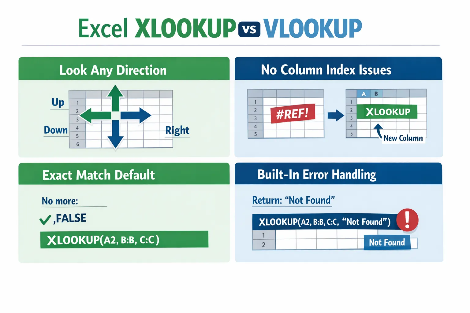
Excel XLOOKUP vs VLOOKUP
- Directional Freedom: It can look left, right, up, or down.
- No Column Counting: You select the specific column you want back. If someone inserts a new column in your sheet, XLOOKUP doesn’t break. VLOOKUP does.
- Exact Match by Default: You no longer have to type FALSE at the end of every formula.
- Integrated Error Handling: It has a built-in “if not found” argument.
How to use xlookup function in Excel
Suppose you are an EdTech administrator. You have a student’s email address, and you want to pull their First Name, Last Name, and Current Grade simultaneously.
- Formula: =XLOOKUP(A2, ‘Students’!E:E, ‘Students’!A:C)
- Result: Because you selected a range of three columns (A:C) as your “return array,” Excel will “spill” all three results into three adjacent cells automatically. This is called a Dynamic Array, and it is the future of Excel.
INDEX & MATCH
Before XLOOKUP, the true elite used INDEX MATCH in Excel. Even today, for users on older versions of Excel or those dealing with massive industrial datasets (over 500,000 rows), INDEX MATCH is often faster and more stable.
- MATCH: This function doesn’t return a value; it returns a position. It tells you that “Product X” is in Row 45.
- INDEX: This function goes to a specific row and column and grabs the data.
How to use INDEX MATCH in Excel with Example:
=INDEX(Vendor_Names, MATCH(Invoice_ID, Invoice_Column, 0))
Beginner Example: Using VLOOKUP to Find Product Prices
Let’s look at a foundational example. Imagine you have a small price list for EdTech software:
| Product ID | Product Name | Price |
|---|---|---|
| 101 | Tally ERP | 18,000 |
| 102 | SAP Business One | 45,000 |
| 103 | Zoho Books | 9,000 |
The Formula: =VLOOKUP(102, A2:C4, 3, FALSE)
How the result is returned:
- Excel searches the first column (Product ID) for 102.
- It finds it in the second row of your data.
- It moves across to the 3rd column (Price).
- It returns 45,000.
For beginners, the key is remembering that the column count includes the starting column.
Common Lookup Errors in Excel and How to Fix Them
Nothing ruins your authority like a spreadsheet full of #N/A errors. Here is how to audit your data like a strategist:
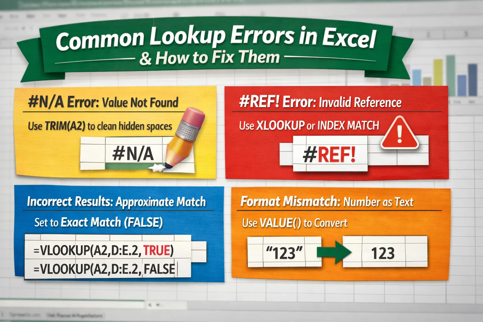
- #N/A Error: The value isn’t found.
- The Fix: Usually, this is caused by hidden spaces. Use =TRIM(A2) inside your formula to clean the lookup value.
- #REF! Error: You deleted a column that the VLOOKUP was pointing to.
- The Fix: Switch to XLOOKUP or INDEX MATCH which use range references rather than hardcoded column numbers.
- Wrong Results: You used TRUE (Approximate Match) instead of FALSE.
- The Fix: In 99% of accounting and EdTech cases, you need an exact match (0 or FALSE).
- Format Mismatch: Looking up a number stored as “Text” in a column of real numbers.
- The Fix: Use the VALUE() or TEXT() functions to ensure both sides of the lookup match in format.
Advanced Lookup Techniques
Intermediate users should master advanced lookup functions in Excel to handle multi-dimensional reporting.
1. Multiple Criteria Lookups
What if you need to find a price for “Widget A” but specifically for the “Western Region”?
- The XLOOKUP Solution: Use the ampersand (&) to join criteria.
- Formula: =XLOOKUP(Cell1 & Cell2, Range1 & Range2, Return_Range)
This effectively creates a unique “virtual key” to find your exact data point.
2. Returning Multiple Results with FILTER
Standard lookups only return the first match. If you need a list of every student who failed a specific subject:
- Formula: =FILTER(Data_Table, Score_Column < 33)
This uses the Dynamic Array engine to return a list of values that automatically shrinks or grows.
3. Wildcard Lookups
If you only have a partial invoice number (e.g., “SAP-101”), you can search using the asterisk:
=XLOOKUP(“*SAP-101*”, Range_A, Range_B, , 2)
The 2 at the end tells XLOOKUP to use wildcard matching.
Industry Use Case: SAP, Tally, and GST Reconciliation
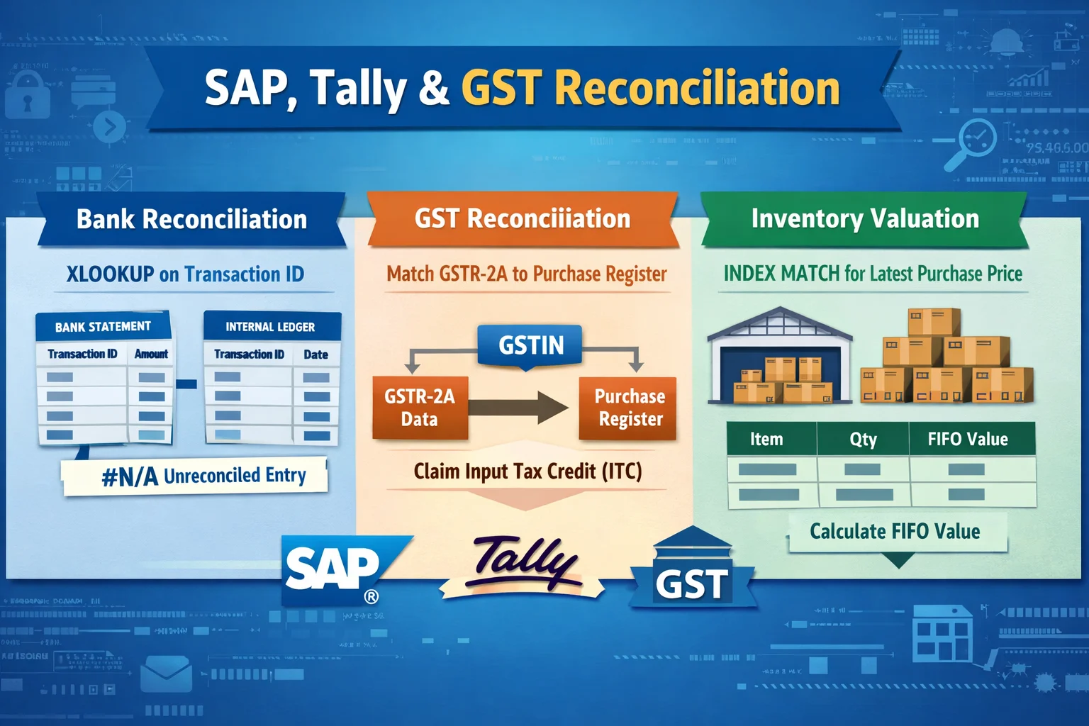
In my years working with Tally, GST, and Industrial accounting, I’ve noticed that lookups are the primary tool for Reconciliation.
- Bank Reconciliation: Use XLOOKUP to match your bank statement’s “Transaction ID” against your internal ledger. Anything that returns #N/A is an unreconciled entry.
- GST Reconciliation: Match GSTR-2A data against your Purchase Register using the GSTIN as the lookup value. This allows you to claim Input Tax Credit (ITC) without missing a single rupee.
- Inventory Valuation: In large manufacturing units, use INDEX MATCH to pull the “Latest Purchase Price” into your current stock sheet to calculate the FIFO (First-In-First-Out) value of your warehouse.
Performance Optimization: Handling 1,000,000 Rows
If your workbook feels laggy every time you press Enter, your lookup functions might be the culprit.
1. Avoid Entire Column References:
Never use A: A. Searching 1,048,576 rows takes processing power. Instead, use a specific range like $A$1:$A$10000 or convert your data into an Excel Table (Ctrl + T) to use structured references.
2. Sorted Data and Binary Search:
If you use VLOOKUP with TRUE (Approximate Match) on a sorted list, it is exponentially faster. This is how the “Big Data” pros handle massive price lists.
3. Move to Power Query:
If you are performing lookups across 10 different files, stop using formulas. Use Power Query (Merge Queries). It is essentially a lookup on steroids that happens in the background, keeping your main Excel file light and fast.
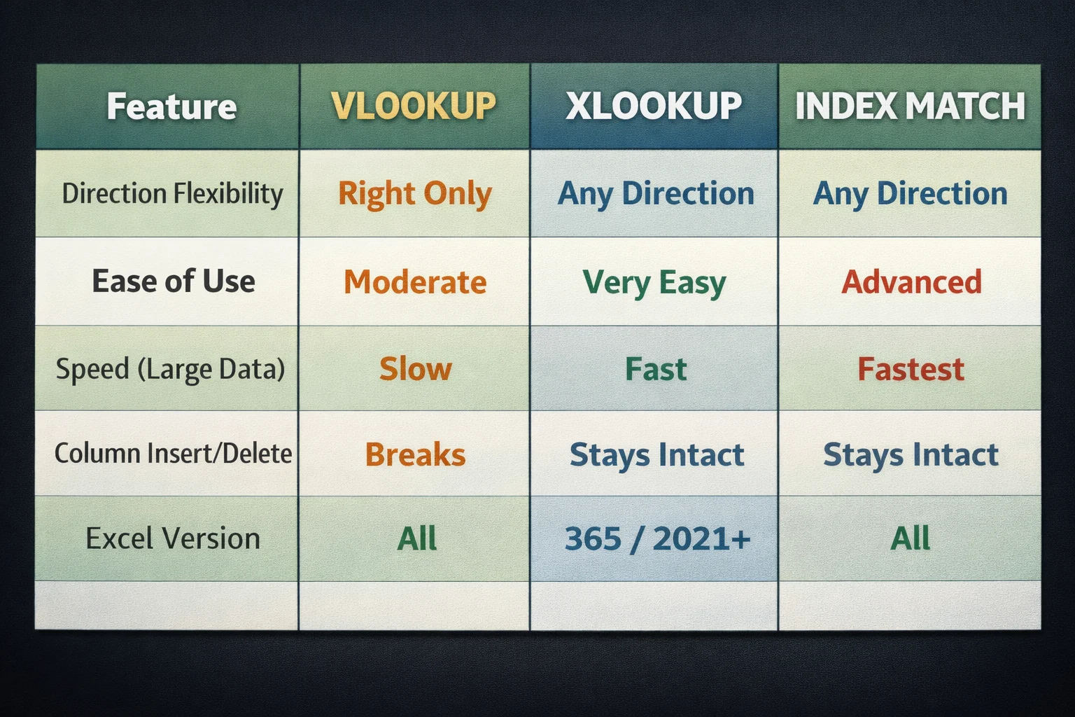
Comparison Table: XLOOKUP vs VLOOKUP vs INDEX MATCH
Conclusion
Mastering How to Use Lookup Functions in Excel is not about memorizing syntax; it’s about understanding how to connect different worlds of data. Whether you choose the classic VLOOKUP or the modern powerhouse XLOOKUP, you are now equipped with the tools to handle any data challenge the EdTech or accounting world throws at you.
Stop manually searching. Start automating. Your time is too valuable for data entry.
Few insightful articles on Excel to improve your knowledge:
Frequently Asked Questions
1. VLOOKUP vs XLOOKUP: Which should I use?
If you are on Excel 365 or 2021, use XLOOKUP. It is easier to write, less prone to errors when columns change, and can look up data to the left. Only use VLOOKUP if you need to share the file with someone using an older version of Excel (2019 or earlier).
2. Why is my lookup returning the wrong value?
This most often happens because you forgot the FALSE or 0 argument for an exact match. Without it, Excel assumes your data is sorted and provides the “nearest” value, which is usually incorrect for IDs or names.
3. Can I look up data in a closed workbook?
VLOOKUP and INDEX MATCH can pull data from a closed file, but the path will become very long. XLOOKUP can also do this, but it is generally safer to use Power Query for cross-workbook data retrieval to avoid “broken link” errors.
4. How do I look up values based on multiple conditions?
The most modern way is using XLOOKUP with ampersands: =XLOOKUP(Criteria1 & Criteria2, Range1 & Range2, ReturnRange). In older versions, you can use a “Helper Column” that combines the two criteria into one.
5. Does VLOOKUP slow down Excel?
Yes, if used excessively over entire columns. To optimize performance, use Excel Tables and limit your search ranges. If your file exceeds 50MB, consider moving your lookups into Power Pivot or Power Query.