
17 Advanced Excel Formulas and Functions: Learn with Real Life Use Cases
Have you heard about Advanced Excel Formulas? These functions can help you perform complex calculations, analyze data, and much more.
Excel has over 450 functions, and I’m sure you’ve heard of popular ones like VLOOKUP, SUMIF, and COUNTIF. You can use these advanced functions alone or combine different functions to create more advanced Excel functions.
Today, most industries are relying on data for better business decisions. To have a good command of data, companies need experts with advanced skills in Microsoft Excel.
If you want to update your skills …..
We’ve gathered the most important and advanced Excel formulas that every top-notch analyst should know.
You can also read more about Advance Excel Courses Online.
If you are interested in becoming an Excel expert like us, you’re going to love this article.
Feel free to download the Excel sheet provided and customize it with your own data.
Table of Contents
1. VLOOKUP Function
Scenario:
Are you a garment shop owner who is always puzzled by their inventory data? Oh!
Let’s see how a garment shop store manager always gives accurate data about their stock items to the shop owner.
The store owner asked him to share the number of shirts left in the stock of all sizes.
As the shop has different varieties of clothes and in them, he has to find several shirts of different sizes. All the inventory data the store manager usually maintains is in Excel.
Manually if he works in Excel to calculate this, it takes a lot of time, and maybe he calculates the wrong numbers.
Then What is the Solution to this problem? Don’t Know! VLOOKUP function that he can use to get results quickly. That’s Why the store manager has to be updated with Excel Advanced Functions.
What is the VLOOKUP() Function?
VLOOKUP(): Here V stands for Vertical. In simple words, it is a function that helps us to search certain data in a column(also called a table array) and then it gives values from different columns but from the same row.
- Lookup_value: The value you want to find in the leftmost column of the range.
- table_array: The range of cells containing the data you want to search through. This range should include both the lookup column and the column where you want to return the result.
- col_index_num: The column number (starting from 1) of the table_array from which you want to retrieve the result.
- range_lookup: Optional. This parameter can be either TRUE (approximate match) or FALSE (exact match). If nothing is mentioned, TRUE is assumed.
How Does VLOOKUP() Function Work?
Let’s see an example of the same store manager to understand how advanced VLOOKUP works. How does he use this function?

Let’s apply Vlookup here in the above Excel data of the garment shop
He is looking for the product shirt and its available size in stock. In the above table, you will see different products listed in column B and their available sizes from Columns C to G.
Formula: =VLOOKUP($B13,$B$5:$G$9, Column(B2),0)
Lookup Value- Shirt
Table Array-B13 (Here we want to find our data) and B5 to G9 (The whole table where the data is searched )
col_index_num: Column B2
range_lookup: 0
$: Here $ is used to fix the value. Generally in Excel, if we want to fix the value of any cell then we use it
Result:
| Product | Small | Medium | Large | XL | XXL |
|---|---|---|---|---|---|
| Shirt | 33 | 51 | 52 | 16 | 28 |
This function of Excel will help him easily search for any data without any errors and save time.
Hope now it’s clear to you how to use advanced Vlookup.
2. XLOOKUP() Function
Scenario:
Let us consider that you are running a cloth shop, for sure you are managing a record of inventory of your stock items. Either you are keeping a record of all these data with any CMS Software or doing it manually with Excel.
If you are managing all this manually then you must be a pro in Excel. But Why?
Here is Why: You need to manage a large record If you will do all these manually then it takes a lot of time to search for any specific products. Here in the example below, a store manager is looking for data on large-size Shirts.
If he will manually find this quantity then it’s time-consuming. Then What is the alternative option for him? XLOOKUP function?
What is the XLOOKUP Function?
The XLOOKUP function in Excel searches a range or array for a specified value and returns the associated value from another column. It can search both vertically and horizontally and perform exact (default), fuzzy (closest), or wildcard (partial) matching.
We will explain the use of match type later on while using the formula. First, we will see how this function works with an example.
- lookup_value: The value you want to find in the lookup_array.
- lookup_array: The range of cells that contains the values you want to search through.
- return_array: The range of cells from which you want to retrieve the result. This range should correspond to the same size as the lookup_array.
- if_not_found: Optional. The value to return if the lookup_value is not found. If omitted, Excel will return an #N/A error.
- match_mode: Optional. This parameter determines whether you want an exact match or the nearest match. Possible values are 0 (exact match), -1 (exact match or smaller), 1 (exact match or larger), or 2 (wildcard match). If omitted, it uses an exact match by default.
- search_mode: Optional. This parameter determines the search direction (1 for vertical, -1 for horizontal) when using an exact match or wildcard match. If omitted, Excel will use a vertical search by default.
How does the XLOOKUP Function work and help the Store manager?
The store manager needs the data on how many large-size shirts are left in the store
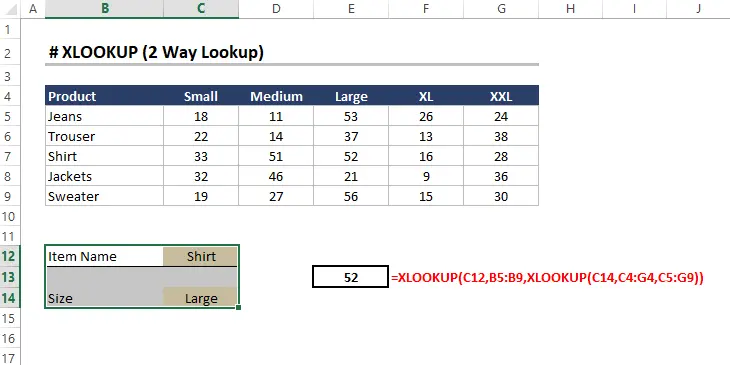
As you can see they have maintained a sheet where products are listed in column B and their different sizes from column C to G. Now the manager is interested to find a shirt(Product) of large size.
Let’s start working with the XLOOKUP() function to get the result of the required query.
Let’s insert this formula into the data mentioned above in the table.
Formula: =XLOOKUP(C12, B5:B9, XLOOKUP(C14, C4:G4, C5:G9))
Lookup Value: Shirt (The product type that we want in our search result)
Lookup Array: B5 to B9 (Here the function searches for our desired product result which is a shirt)
Return Array: C12( Here we want to find our data on the sheet of product shirt)
Again XLOOKUP is applied
Lookup Value: Large Size (The product size type that we want in our search result)
Lookup Array: C4 to G4 (Here the function searches for our desired result which is a large shirt size type that is Large)
Lookup Array: C5 to G9 (Here the function searches for our desired result which is a shirt-specific size that is 52 as mentioned in the result)
Return Array: C14 ( Here we want to find our data on the sheet of product shirt size)
The other parameters that are mentioned above are optional. It means we can add them if we want or else we can avoid them.
Result:
| Item Name | Shirt | |
| Size | Large
|
The desired output is 52 large-size shirts quantity.
This function provides a two-way lookup which means both horizontal and vertical. It is more flexible than Vlookup and Hlookup. Thus it increases efficiency and productivity.
We tried to explain it more simply with examples so that it is clear for you. Hope you found this helpful.
How is XLOOKUP Better than VLOOKUP?

There are many more functions available in XLOOKUP in comparison to VLOOKUP. You can check below:
3. IF | IF OR | IF AND Function
Scenario:
When you are leading a finance team of a big company and have to manage large records of data. Sometimes it seems complex to manage accurately.
Mahesh a finance Team Leader at a big MNC has been asked to submit a report on salary hikes in different departments.
Now, He is tense because the company operates in a different location and there are a lot of departments and many other things there.
What is the Solution to his problem, if he already has a sheet with different data as mentioned below in the example?
He can use the If function, and If OR function to find the required results as per the conditions described to him. Why did he use this function? It helps him to get the desired data quickly and with 100% accuracy.
What is the IF() Function?
The advanced IF function in Excel allows you to perform conditional evaluations and return different values based on a specified condition. It is widely used for logical and decision-making purposes in spreadsheets.
- logical_test: This is the condition you want to check. It can be any logical expression that evaluates to either TRUE or FALSE.
- value_if_true: The value to be returned if the logical_test evaluates to TRUE.
- value_if_false: The value to be returned if the logical_test evaluates to FALSE
We will discuss first the IF function and then move to IF OR and IF AND with the same example.
How Does IF Function Work?
Let’s go through an example to understand how the IF function works and help Mahesh
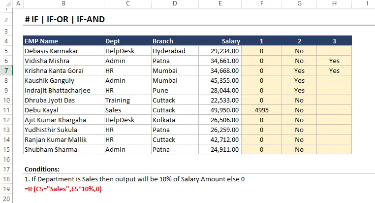
Here in the above example, you can see in the table Employee’s name is mentioned in Column B. Their department is in Column C, the Branch is in Column C, and salary data is in Column E.
Now here Mahesh wants to find if (the department is sales then the output will be 10% of the Salary Amount else 0)
Formula: =IF(C5=” sales”, E5*10%,0)
Logical Test: If the department is sales (C5= “sales”)
Value if True: Output will be 10% of the salary
Here, salary is mentioned in column E, and for sales, it is E5 so the output will be E5*10%
Value If False: If the department is not sales then return the value zero(0)
Result:
As you can see below the result is displayed in column 1. For sales, it displays a value of 4995 and for the rest, it shows 0
Now, we will move toward the
IF-OR function
- condition1, condition2, etc.: These are the multiple conditions you want to check. They can be any logical expressions that evaluate to either TRUE or FALSE.
- value_if_true: The value to be returned if any of the specified conditions evaluate to TRUE.
- value_if_false: The value to be returned if all of the specified conditions are evaluated as FALSE.
Now Mahesh wants to find if the branch is Mumbai or Branch is Pune then the output will be Yes else No
Formula: IF(OR(D5= ”Mumbai”, D5=” Pune”),” Yes”,” No”)
Here the branches are available in Column D
Condition 1: If the Branch is Mumbai (D5=Mumbai)
Condition 2: If the Branch is Pune (D5=Pune)
Value_if_True: Yes
Value_if_False: No
Result:
The desired result is mentioned above in the image as you can see.
The last one is
If And Function
- condition1, condition2, etc.: These are the multiple conditions you want to check. They can be any logical expressions that evaluate to either TRUE or FALSE.
- value_if_true: The value to be returned if all of the specified conditions evaluate to TRUE.
- value_if_false: The value to be returned if any of the specified conditions are evaluated as FALSE.
Let’s see this with an example, Mahesh’s Manager now asked him to share the salary data of employees.
But for that employee only whose salary is between 30000-35000.
Mahesh can use if and function then easily he can get the required data.
If the Salary is between 30000 and 35000 then the output will be Yes else Blank cell
Formula: IF(AND(E5>=30000, E5<=35000)” YES”,” “)
Below is the image you can see in the third column that is representing this data
Still, if you have any doubts then you can join MS Excel Course
4. SUMIF() Function
Scenario:
Have you read the previous scenario of Mahesh?
Again Mahesh’s Manager has asked him to submit the annual salary report of different departments.
As Mahesh is maintaining an Excel sheet of all data but it’s too difficult for him to calculate manually.
Then What? Mahesh will submit the requested report on time or he do the manual calculation.
Mahesh is too smart. Want to know How? He used the SUMIF() function to do this task.
What is SUMIF() Function?
The SUMIF() function in Excel is used to sum values based on a specified condition or criteria. It allows you to add up values that meet a specific requirement.
- range: This is the range of cells you want to evaluate against the criteria. It is the range that will be checked for the condition.
- Criteria: This is the condition that you want to apply to the cells in the range. It can be a number, text, expression, or cell reference.
- sum_range (optional): This is the range of cells that you want to sum up if their corresponding cells in the range meet the criteria. If not provided, the function will use the same range as the range parameter for the summation.
How Does SUMIF() Function Work?
Now see how smartly Mahesh uses this function to prepare the final report.
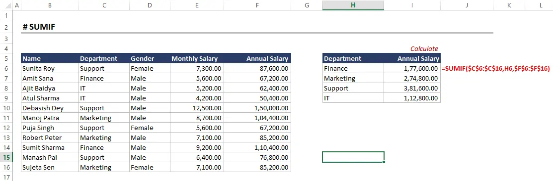
Let’s apply the function to the above data
Formula: =SUMIF($C$6: $C$16, H6, $F$6: $F$16)
Range: C6 to C16 ( Here he wants to apply the function against the mentioned Criteria)
Criteria: Finance, Marketing, Support, IT ( This is the criteria against which we want our sum data)
Sum_range: F6 TO F16 (This is the range of salary data (column F) that will be summed up in their corresponding cells in column C to meet the criteria)
Result:
| Department | Salary |
|---|---|
| Finance | 1,77,600.00 |
| Marketing | 2,74,800.00 |
| Support | 3,81,600.00 |
| IT | 1,12,800.00 |
5. OFFSET + SUM Function
Scenario:
Joy is running a Toy Shop due to some reasons he is not coming to shop for a few days (03.07.2023 – 13.07.2023)
When Joy is back to work he asks the Store Manager who is handling all his work in his absence. To show the data of total toy sales quantity.
Now, the Store Manager has already prepared the sheet that contains date-wise sales quantity. But now he is worried that he has to calculate the total sales quantity manually.
Is there any other option to calculate this? The answer is “Yes” Store managers can use OFFSET+SUM advanced Excel function to do this task.
What is the OFFSET + SUM Function?
The OFFSET + SUM combination in Excel allows you to create a dynamic range and then sum the values within that range. The OFFSET function helps define a new range based on a starting point, and the SUM function then adds up the values within that new range. This combination is useful when you need to perform calculations on a changing range of cells.
- Reference: This is the starting cell from which the new range will be defined.
- rows: This is the number of rows to move from the reference cell to determine the starting row of the new range. It can be a positive or negative value.
- cols: This is the number of columns to move from the reference cell to determine the starting column of the new range. It can be a positive or negative value.
- height (optional): This is the number of rows in the new range. If not specified, the new range will be one cell high.
- Width (optional): This is the number of columns in the new range. If not specified, the new range will be one cell-wide.
How Does OFFSET + SUM Function Work?
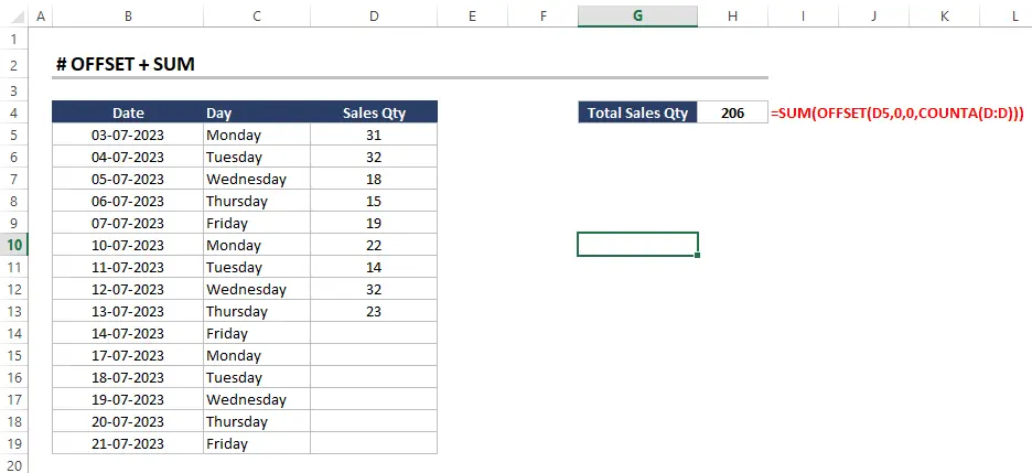
Formula: =SUM(OFFSET(D5,0,0, COUNTA(D:D)))
Reference: D5(This is the reference cell, which is the starting point for the new range.)
Rows: CountA(D:D) (This part of the formula calculates the number of rows to move up from the last cell in column D (13.07.2023) to reach the first cell of the new range (03.07.2023.)
The OFFSET function will create a new range representing the sales figures. After that SUM function sums up the sales values within the new range.
Once the store Manager applies this formula to the above data he will get the result of exact sales from 03.07.2023 to 13.07.2023
Result:
| Total Sales Quantity | 206 |
|---|
The next function in the Advance Excel Formula list is COUNTA(). Let’s dive into this with real-life scenarios.
6. COUNTA() Function
Scenario:
Let’s consider you are running a restaurant business and a few days back you hired a manager to manage all the staff.
Once the manager has joined the restaurant, he wants to know the total no of staff currently working.
Now as an owner, you handed him all the Excel records of the Staff data and told him to get the details from this.
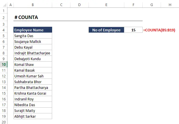
The manager is so smart that he quickly applies the COUNTA() Function in the Excel sheet and gets the results—the total no of staff working in the restaurant.
As an owner, you can also learn advanced Excel Functions. Let’s start first with What the is COUNTA Function and how the manager uses this function also.
What is COUNTA() Function?
The COUNTA function in Excel Formula is used to count the number of cells in a range that are not empty. It includes both numerical values and text entries, making it useful for counting non-blank cells.
value1, value2, etc.: These are the arguments representing the cells or values you want to count. You can provide up to 255 arguments.
How Does COUNTA() Function Work?
Just apply the above-mentioned formula
Formula: =CountA(B5:B19)
Result:
| No of Employee | 15 |
|---|
The COUNTA() function is particularly useful for data analysis tasks, where you need to determine the number of cells with data
Here you can see how a manager can easily calculate the staff number which is 15.
This advanced Excel formula makes it easy for the Manager to count staff no. Even the owner is also impressed.
7. COUNTIF() Function
Scenario:
Let’s walk through a case in which you are working in a company as an HR Executive. Recently your upper management asked you to submit a report on the total no of employees in each respective department.
Now What is the option you have to calculate this
-
- Manually
- Use Excel Functions
Which works best with maximum productivity and efficiency the answer is Excel Function.
Which Excel function you can use to prepare the report “COUNTIF() function”? But many are still not aware of this function and How to use it.
Don’t Worry! We are here to explain.
What is the COUNTIF() Function?
The COUNTIF() function in Excel is used to count the number of cells within a range that meets a specified criterion. It allows you to count cells based on specific conditions or criteria.
- Range: This is the range of cells you want to evaluate against the criteria. It is the range that will be checked for the condition.
- Criteria: This is the condition that you want to apply to the cells in the range. It can be a number, text, expression, or cell reference.
How Does COUNTIF Function Work?

As you can see in the above image there is a complete employee details sheet.
Let’s start working with this sheet to get the total no of employees in different departments. Apply the formula
Formula: =COUNTIF($C$6:$C$16, H6)
Range: C6 to C16 ( Here we want our criteria to be checked)
Criteria: You have selected the different departments like Finance, Marketing, Support, and IT.
When you apply the formula to your data. The following result you get
Result:
| Department | No of Employee |
|---|---|
| Finance | 2 |
| Marketing | 3 |
| Support | 4 |
| IT | 2 |
Hope this information helps you to improve your Excel Knowledge.
If you are interested to explore more about MS Office then check below
Explore more about MS Office
All-Purpose Benefits Of Microsoft Office Specialist Certification Courses
Top 10 Techniques | Microsoft Advanced Excel Certifications
8. MATCH() Function
Scenario:
Let us explore an example that you are working in a bank. Your branch manager asked you to find a position of the Transaction ID of a customer from the Excel sheet report.
The manager mentioned to you that he needs this urgently because there is some issue with that customer’s bank account.
Now if you will start finding this from your large data sheet manually. It means you can not submit the details to the manager on time. So, you have to work smartly here, you can use the MATCH() function.
What is the MATCH() Function?
The MATCH() function in Excel allows you to find the position of a specified value within a range. It is commonly used in combination with other functions like INDEX() to perform advanced lookup and retrieval operations.
-
- lookup_value: This is the value you want to find within the lookup_array.
- lookup_array: This is the range or array in which you want to search for the lookup_value.
- match_type (optional): This parameter specifies the type of matching to be performed. It can be one of the following values:
- 1 (or omitted): Finds the largest value less than or equal to the lookup_value (default).
- 0: Finds the first exact match to the lookup_value. The lookup_array must be sorted in ascending order.
- -1: Finds the smallest value greater than or equal to the lookup_value. The lookup_array must be sorted in descending order.
How Does the MATCH() Function Work?
When you apply the formula in your data sheet you can easily find the result. Check below how it will help you.
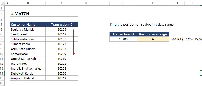
Formula: MATCH(F7, C5:C15,0)
Lookup Value: 10209 (This is the value we want to find in the lookup_array)
Lookup Array: C5:C15 (This is the range or array in which we want to search for “10209.”)
Match Type: 0 (The match_type is set to 0 to find the first exact match)
After applying the formula see how easily you can get the result
Result:
| Transition ID | Range |
|---|---|
| 10209 | 6 |
9. INDEX+ MATCH /VLOOKUP + CHOOSE Function
Scenario:
Hopefully, you have read the previous scenario of the bank. What if the manager again asked to find the customer name also with the Transaction ID?
Confused! How can you search for this requested information?
Why are you worried if we are here to help you?
There are two different types of functions you can use to get this result
INDEX+ MATCH Function VLOOKUP + CHOOSE Function
What is the INDEX+ MATCH Function?
The combination of INDEX and MATCH functions in Excel is a powerful way to look up and retrieve specific data from a table.
The INDEX function returns the value of a cell in a specified row and column within a range. While the MATCH function is used to find the position of a lookup value within a given range.
When used together, they allow you to perform a two-dimensional lookup, where you can find a value based on both row and column criteria.
Formula (MATCH Function): MATCH(lookup_value, lookup_array, [match_type])
- array: This is the range or array from which you want to retrieve the data.
- row_num: This is the row number from which you want to get the value.
- column_num (optional): This is the column number from which you want to get the value. If omitted, the function returns the value from the specified row only.
- lookup_value: This is the value you want to find within the lookup_array.
- lookup_array: This is the range or array in which you want to search for the lookup_value.
- match_type (optional): This parameter specifies the type of matching to be performed
How Does the INDEX + MATCH Function Work?
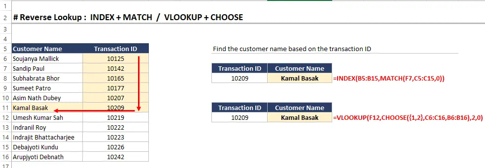
Formula(INDEX + MATCH): INDEX(B5:B15, MATCH(F7, C5:C15,0))
Array: B5:B15 (This is the array from which you want to retrieve the data).
Row_num: F7 (This is the row number (Customer ID) you want from the MATCH function.)
Lookup Value: Customer Name (The name of the customer you want as per the Transition ID)
Lookup Array: C5:C15 (This is the range or array in which you want to search for the customer name).
Match Type :0
After successfully applying the formula your result will be there in a fraction of a second.
Result:
| Transaction ID | Customer Name |
|---|---|
| 10209 | Kamal Basak |
This is the first way to find the required details. Let’s see another option in detail
VLOOKUP + CHOOSE Function
What is the VLOOKUP + CHOOSE Function?
The combination of VLOOKUP and CHOOSE functions in Excel allows you to perform more complex lookups and get data from different columns based on a single criterion.
The VLOOKUP function looks for a value in the leftmost column of a range and returns a corresponding value from a specified column within that range.
The CHOOSE function allows you to select a value from a list of values based on a numeric index. When used together, you can dynamically choose which column to look up the data based on the result of another function.
- lookup_value: This is the value you want to find in the leftmost column of the table_array.
- table_array: This is the range or array containing the data to be searched. The lookup_value should be in the leftmost column of this range.
- col_index_num: This is the column number within the table_array from which the result should be returned.
- range_lookup (optional): This parameter is either TRUE (approximate match) or FALSE (exact match). If omitted, it defaults to TRUE.
- index_num: This is the numeric index that specifies which value to select from the list of values provided in the CHOOSE function.
- value1, value2, etc.: These are the values from which you want to choose based on the index_num.
Now, we will discuss how this function works and reduce the workload.
How Does the VLOOKUP + CHOOSE Function Work?
Formula: VLOOKUP(F12, CHOOSE({1,2}, C6:C16, B6:B16),2,0)
Lookup Value: Customer Name
Table Array: B6 to B16
Col_index_num: F12
The following result will be displayed
Result:
| Transaction ID | Customer Name |
|---|---|
| 10209 | Kamal Basak |
This combined function helps you to perform lookups based on different criteria. Then you can choose which data you want.
Still facing issues with the basic concepts of advanced Excel formulas and functions. No need to worry more because ICA Experts have designed the full course on MS Office that covers the Advanced Excel Function Class.
10. CONCATENATE() Function
Scenario:
A school Class teacher is maintaining a student name list in Excel. Firstly he used to maintain his First Name in one column and his Second Name in another column.
Later on, the Principal asked to reframe the list and include their name in only one Column. It means both first and second names combined written.
As per instructions class teacher started preparing the revised sheet but he is doing it manually one by one.
Do you have any idea about any Excel function that can complete this task in a short time?
No, We will tell you How you can do this. It’s so simple just use the CONCATENATE function in Excel.
What is a CONCATENATE Function?
The CONCATENATE function in Excel is used to combine multiple text strings into a single string. It allows you to join together the contents of two or more cells or add additional text or characters in between the cell values
text1, text2, etc.: These are the text strings or cell references that you want to concatenate. You can include up to 255 text strings or cell references.
How Does the CONCATENATE Function Work?
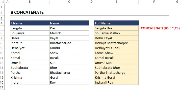
Formula: =CONCATENATE(B5, “ “, C5)
After applying the formula to the student name list. You can get the result like this:
Result:
| Full Name |
|---|
| Sangita Das |
| Soujanya Mallick |
| Debu Kayal |
| Indrajit Bhattacharjee |
| Debajyoti Kundu |
| Komal Shaw |
| Kamal Basak |
| Umesh Sah |
| Subhabrata Bhor |
| Partha Bhattacharya |
| Krishna Gorai |
| Indrani Roy |
11. REPT() Function
Scenario:
Let’s move with an example where HR has been advised to prepare the review rating sheet of the employee.
After receiving the details from the manager, HR started preparing the sheet. However, the manager has advised HR to mention * as a string with the respective rating number of employees.
HR as per instructions wrote * manually after each rating no in the next column. But, it’s too time-consuming matter.
So, HR asked his colleagues to suggest some alternative options for this. His colleague suggested using the REPT Function.
What is REPT Function?
The REPT() function in Excel allows you to repeat a text string a specified number of times. It is useful for creating repeated patterns or generating repetitive text values.
-
- Text: The text string that you want to repeat.
- number_times: The number of times that you want to repeat the text string.
How Does the REPT Function Work?

Formula: =Rept(“*”, C5)
Text: * (This string is inserted repetitively).
Number_times: Number of times we want * to be repeated in the sheet.
Once this formula is applied, it generates the text string of each rating number.
For example, It writes 5 times * for Sangita Das. As she got a 5 rating.
Result:
In the above image, you can see that * is written as the no of times a numerical value is given to it.
12. TYPE() Function
Scenario:
Let’s move with an example in which a student has been asked to differentiate the data mentioned on the Excel sheet based on a numerical value.
The teacher has given him the Excel sheet and the information on the numerical value according to the data type
As per the instruction by the teacher, the student started preparing the sheet. In the beginning, manually he is doing this task.
He is checking the pre-given information that if data is a number then write 1. If the data is text then write 2.
Later on, when he did not submit the task on time. One of his friends told him to use the TYPE function to complete the assignment.
What is the TYPE Function?
The TYPE() function in Excel allows you to determine the type of data contained within a cell. It returns a numerical code that corresponds to a specific data type. This function is useful when you need to identify the type of data stored in a cell or a formula result.
-
- Value: The cell reference or the value that you want to determine the type of.
The TYPE function returns the following numerical codes for different data types:
-
- 1: Number
- 2: Text
- 4: Logical (Boolean)
- 16: Error
- 64: Array
- 128: Cell reference
How Does the TYPE Function Work?
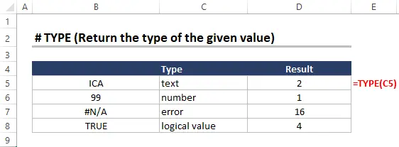
Formula: =TYPE(C5)
When the formula is applied to the above data, it represents the numerical value according to the type of inserted data.
For example, For the text, ICA shows the value of 2 because ICA comes under the text category.
Result:
You can see in the above image how easily one can determine the type of data value with the help of the Type function.
13. LEFT_MID_RIGHT Function
Scenario:
Let’s start with the simple example of a Guest House. There is a conference organized by the local administration of the city in Hotel Paris
As per the instructions from the local administration, the hotel has to prepare a sheet of guest list with few details. The guest list sheet contains
-
- Start Code ( Given by the local administration)
- PAN ( PAN ID of Guests)
- Last 3 ( A unique code hotel has given to their guests.)
Now at the end of the conference, the hotel authorities have to submit all these details to local administrations.
By mistake, at the time of writing guest details, they had written all these details combined in one column. However, they have been advised to submit it in three separate columns.
So, now what they can do to separate these details? They can use LEFT_MID_RIGHT Function.
What is LEFT_MID_RIGHT Function?
The LEFT, MID, and RIGHT functions in Excel are used to extract parts of a text string. The LEFT function extracts the first n characters from a text string, the MID function extracts a specified number of characters from a text string starting at a specified position, and the RIGHT function extracts the last n characters from a text string.
The LEFT, MID, and RIGHT functions are all very similar, but they have some key differences.
The LEFT function always extracts the first n characters from a text string, regardless of where the nth character is located.
The MID function extracts a specified number of characters from a text string starting at a specified position. The position can be specified as an absolute position or as a relative position.
The RIGHT function extracts the last n characters from a text string.
How Does the LEFT_MID_RIGHT Function Work?

Let’s apply these three functions in the above image of the datasheet of guest list details
We will apply all the formulas in column B where GSTIN (Unique ID List created by the hotel) is written.
So, When we apply the LEFT function it displays the result as START CODE
= LEFT(B6,2)
Here we have selected the complete B column starting from 6, and the first two digit number it displays from the text string
After that apply the function MID
=MID(B6,3,10)
Here we have selected Column B and from this, it selects from 3 characters to 10 characters from the text string.
The last one is the RIGHT Function
=RIGHT(B6,3)
Here we have selected Column B and the last 3 characters will display
Results:
You can see the result of all three functions in the above image as Start Code, PAN, and Last 3.
Hope now you can use these functions easily whenever you need to separate the details from text strings.
How easily one can implement these advanced Excel functions for data analysis? It makes their work easy and improves efficiency.
You can explore here more about Advance Excel Courses.
14. RANDBETWEEN() Function
Scenario:
Let’s imagine you are running a promotional campaign for an online store. You want to offer random discounts to customers as an offer to attract them to purchase your products.
You have decided to offer discounts between 5% and 20% off on their total purchase amount.
Now you have to create the sheet where you will add discounts for customers. If you will prepare the discount sheet manually for customers it takes a lot of your time.
So, How do you manage this situation?
You can use the RANDBETWEEN function in Excel to generate random discount values within 5% to 20%. Based on the percentage discount then you can calculate the discounted amount on their total bill.
What is RANDBETWEEN Function?
The RANDBETWEEN function in Excel generates a random number between two numbers that you specify.
-
- lower_bound: The smallest number that the function can return.
- upper_bound: The largest number that the function can return.
The RANDBETWEEN function will always return a number that is greater than or equal to the lower_bound and less than or equal to the upper_bound
How Does the RANDBETWEEN Function Work?
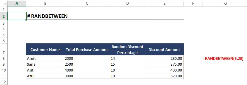
Formula: =RANDBETWEEN(5,20)
Let’s apply this formula in the above datasheet.
Lower Bound: 5% ( It means the minimum discount that can be given to customers is 5% on their purchase)
Upper Bound: 20%(It means the maximum discount that can be given to customers is 20% on their purchase)
In cell D2 (the first row under “Random Discount Percentage”), enter the formula =RANDBETWEEN(5, 20). This will generate a random whole number between 5 and 20 as the discount percentage for the first customer.
To calculate the discounted amount for each customer, use the formula =[@’Total Purchase Amount’] * (1 – [@’Random Discount Percentage’]/100) in cell D2 (the first row under “Discounted Amount”). This formula will calculate the discounted amount based on the respective customer’s total purchase amount and random discount percentage.
Result:
You can see in the above image that after applying the formula random discount for each customer is generated. After that discounted amount is calculated. All the discount percentages are between 5 to 20.
15. CONVERT() Function
Scenario:
There is one grocery shop that maintains the weight data of all the sold products in kg.
But the shop owner is too concerned about the weight and he doesn’t want to miss a single gram of any product.
So, he decided to maintain one more column in Gram. But he is not in the mood to do this manually at all one by one.
He called his son and asked, Is there any advanced Excel function that could automatically convert the measurement details. His son replied Yes “Dad” You can use the CONVERT function.
What is CONVERT Function?
The CONVERT() function in Excel is a powerful tool for unit conversion. It allows you to convert a value from one measurement unit to another.
-
- Number: The number that you want to convert.
- from_base: The base of the number that you want to convert from.
- to_base: The base of the number that you want to convert to.
How Does the CONVERT Function Work?
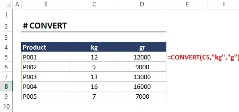
Formula: =CONVERT(C5,” kg”,g”)
Number: C5 (The kg column that we want to convert)
From_base: Kg(The base of the number that we want to convert from).
To_base g(The base of the number that we want to convert to).
When we apply the above formula it will convert all the measurements from Kilogram(kg) to gram(g).
Result:
You can see in the above image where the final data on converted product weight is written in gram(g)
We are trying to explain each advanced Excel formula with examples so that you can better understand the concepts.
But if you want more information and are interested to learn more join the Advance Excel Formula Course.
16. SUMPRODUCT() Function
Scenario:
Just imagine you are running a stationary shop. For each day of sales of the most expensive product of your store, you are maintaining a sheet with product quantity sold with their prize.
From Monday to Saturday, you are maintaining this sheet so that you can calculate the total sales of the most expensive item. Now on Sunday, you are calculating final sales but have no idea how to do this quickly instead of one by one.
You searched on Google and Google answered you to use the SUMPRODUCT function.
What is SUMPRODUCT Function?
The SUMPRODUCT() function in Excel is a versatile tool for performing calculations on arrays or ranges. It allows you to multiply corresponding values in multiple arrays or ranges and then sum the products.
-
- array1: The first array.
- array2: The second array.
- …: Additional arrays.
How Does the SUMPRODUCT Function Work?
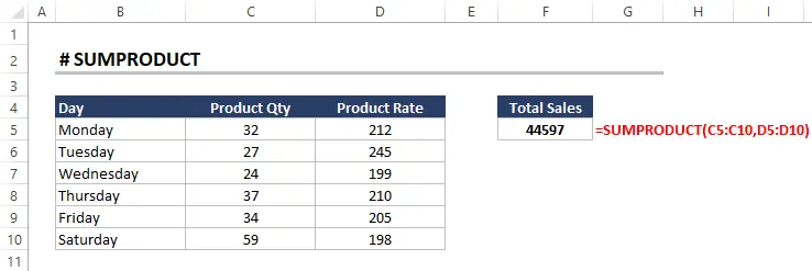
Formula: =SUMPRODUCT(C5:C10, D5:D10)
-
- array1: C5: C10 (The first array of data that we want to multiply)
- array2: D5:D10 The second array of data from which the first array is multiplied)
After that final result is the sum of all the multiplied values.
For Example C5* D5 + C6*D6 + ……
Result:
| Total Sales |
|---|
| 44597 |
See, it’s so easy. We hope you can do this type of calculation by using this formula.
17. IFERROR() Function
Scenario:
Maria works in a Cosmetic shop as sales Person. The cosmetic shop owner once asked Maria to prepare a report on the average sales price of all products.
The owner also suggested to Maria that if there is any product in the stock whose sales are 0. Then mention that in the sheet and give a 0 value to that product in the list.
Maria started preparing the sheet smartly by using the IFERROR Function.
Are you interested to know more about this Excel Function? Let’s dive into this
What is the IFERROR Function?
The IFERROR() function in Excel allows you to handle and manage errors in formulas. It helps you control the output or display a specific value when an error occurs. In simple words 1
The IFERROR function in Excel returns a value you specify if a formula evaluates to an error; otherwise, it returns the result of the formula
- formula: The formula that you want to check for errors.
- value_if_error: The value that you want to return if the formula evaluates to an error.
How Does the IFERROR Function Work?

Formula = IFERROR(B14/C14,0)
Let’s evaluate the data sheet with the IFERROR function.
In the above image of the first datasheet, as you can see, the average value(Avg Price) is calculated by dividing the total sales by the total quantity(B5/C5)
In the second datasheet of the same image when we apply the IFERROR function it evaluates. if the average price is B14/C14 is correct then the result value is written else displays 0 as an error.
It helps Maria to easily identify products with sales. Also, it fulfills the requirements of the shop owner.
For example, There is one product with a sales value of 747 and a quantity of zero. It means no product with that sales value is sold. Thus while calculating its average price, it shows an error.
When, Maria finally prepared the sheet and applied the IFERROR function, that particular sales value results will show an average price of zero. (According to the condition used by Maria)
Result:
In the above image you can check the result of the applied function>
Conclusion:
In the End…
If you’re tired of doing things manually and want to use the advanced formula of Excel. Then you are in the right place.
You can learn the complete advanced Excel formula from experts.
By using these Advanced Excel Functions you can increase your productivity and save a lot of time. We have tried to cover all the important Excel Formulas that is widely used by data scientist. To make things easy to understand, we have used a real-life example that helps you to clear your basic concepts.
Whether you are a business professional, a student, or a data analyst these formulas will help you. Excel functions have the power to make your work processes easy and unlock valuable insights from your data.

Debjit Chakraborty
Certification : Certified Microsoft Excel Expert and Tally Profession: Ms Excel, TallyPrime Trainer Organization: Corporate Trainer – Technical Quality Assurance at “ICA Edu Skills Pvt. Ltd".
Industry Experience :Expert of MS Office and Tally, with over 16+ years of experience, trained more than 7,000+ individuals and Delivered Master Classes for over 100+ trainers of Excel and Tally. Mr. Debjit Chakraborty has a rich experience in training for over 16+ years. He has trained over 7,000+ students and over 100+ trainers of Excel and Tally.
Linkedin Profile:https://in.linkedin.com/in/debjit-chakraborty-873b6887