Custom Number Formatting In Excel: Ways To Create & Apply
The concept of custom number formatting in Excel is quite tricky in nature and it can become difficult for you if you are not aware of it. This feature of Excel allows users to format all the time, date, and text in specific ways. Most importantly it goes beyond the default option.
Whenever you define all the custom number formats you can make use of the combination of codes, symbols, and placeholders. It is one of the crucial aspects of the number formatting in Excel.
It only affects the way the numbers are displayed but it does not affect all the underlying values of the numbers. So, let’s explore the facts to have a clear insight to it.
Table of Contents
- What Is Custom Number Formatting In Excel?
- What Can You Do With Custom Number Formats?
- Basics Of Custom Number Formatting
- Common Custom Format Symbols
- Where To Use Custom Number Formats?
- How Custom Number Formatting Works In Excel
- How To Apply Custom Number Formatting
- Benefits Of Using Custom Number Formats
- Where Can You Find The Number Formats
- Problems & Possible Solutions
- What Are The Common Shortcuts For Number Formats
- Different Ways To Format Numbers In Excel
- FAQ(Frequently Asked Questions)
- Final Takeaway
What Is Custom Number Formatting In Excel?
Custom number formatting in Excel allows you to create and apply your own display formats for numbers, dates, times, and text in cells without altering the underlying data. It controls how values appear in a worksheet, enabling you to tailor appearances for better readability or specific requirements, such as adding units, symbols, or conditional displays.
What Can You Do With Custom Number Formats?
Custom number formatting in Excel lets you control how numbers, dates, times, and text are displayed in cells without changing the underlying data. Here’s what you can do with them:
1. Customize Number Displays
- Add Units or Labels: Append text like “kg”, “USD”, or “%” to numbers (e.g., 0.00 “kg” displays 5.00 kg for 5).
- Control Decimal Places: Show specific decimal places (e.g., 0.00 ensures two decimals, like 123.45).
- Include Thousands Separators: Use commas for readability (e.g., #,##0 displays 1,234 for 1234).
- Hide Insignificant Zeros: Use # to skip unnecessary zeros (e.g., ###.## shows 123.4 instead of 123.40).
- Align Decimals: Use ? to align numbers with varying decimal places (e.g., 0.?? aligns 1.2 and 1.23).
2. Format Positive, Negative, Zero, and Text Differently
- Use a four-part format: Positive;Negative;Zero;Text (separated by semicolons).
- Example: #,##0.00;[Red]-#,##0.00;0.00;”Text”@ shows:
- Positive: 1,234.00
- Negative: -1,234.00 in red
- Zero: 0.00
- Text: Text followed by the input text.
- Example: #,##0.00;[Red]-#,##0.00;0.00;”Text”@ shows:
- Display negatives in parentheses or custom colors (e.g., $#,##0;($#,##0) shows ($1,234) for -1234). It is one of the crucial aspects of custom number formatting in Excel.
3. Customize Dates and Times
- Create specific date formats (e.g., dd-mmm-yyyy shows 02-Aug-2025).
- Show only parts of a date (e.g., mmmm yyyy displays August 2025).
- Format times (e.g., hh:mm AM/PM shows 11:15 AM).
- Combine date and time (e.g., dd-mmm-yy hh:mm shows 02-Aug-25 11:15).
4. Create Conditional Displays
- Apply formats based on value ranges using conditions like [>1000]#,##0;”Small”.
- Example: [>1000]#,##0;”Small” shows 1,234 for 1234 and Small for values ≤1000.
- Use colors for conditions (e.g., [Green][>=100]#,##0;[Red]#,##0 for green if ≥100, red otherwise).
5. Format Special Numbers
- Phone Numbers: Use (###) ###-#### to display 1234567890 as (123) 456-7890.
- ZIP Codes: Use 00000 to ensure five digits (e.g., 00543 for 543).

Basics Of Custom Number Formatting
Custom number formatting in Excel lets you control how numbers, dates, times, and text appear in cells without changing their actual values. It’s a way to make data more readable or fit specific needs using custom format codes. Below are the basics to get you started.
Core Components
Custom formats use specific symbols to define how data is displayed. A format can have up to four sections, separated by semicolons: Positive;Negative;Zero;Text.
Key Symbols
0: Shows a digit, including insignificant zeros (e.g., 00 displays 05 for 5).
#: Shows significant digits only (e.g., ## displays 5 for 5, no leading zeros).
?: Adds spaces for alignment, often for decimals or fractions (e.g., 0.?? aligns 1.2 and 1.23).
.: Decimal point (e.g., 0.00 shows two decimal places).
,: Thousands separator (e.g., #,##0 displays 1,234).
%: Displays numbers as percentages (e.g., 0% shows 50% for 0.5).
/: For fractions (e.g., # ?/? shows 3 1/2 for 3.5).
$, €, etc.: Adds currency symbols or custom text (e.g., 0 “kg” shows 5 kg).
@: Represents text in a cell (e.g., “Text: “@ shows Text: ABC for “ABC”).
[Color]: Applies colors (e.g., [Red] for negative numbers).
Structure Of Custom Format
Four Sections: Positive;Negative;Zero;Text
- Example: #,##0;[Red]-#,##0;0;”Text”@
- Positive: 1,234
- Negative: -1,234 in red
- Zero: 0
- Text: Text followed by input text
- If fewer sections are specified, Excel applies defaults (e.g., #,##0;-#,##0 covers positive and negative, with zeros and text using default formats).
Common Custom Format Symbols
There are some of the common custom format symbols that you must be well aware of while you want to make use of these symbols. So, let’s find out some of the crucial facts that can make things happen in your way.
- 0: Displays a digit, including insignificant zeros (e.g., 00 shows 05 for 5).
- #: Displays significant digits only, omitting insignificant zeros (e.g., ## shows 5 for 5, no leading zeros).
- ?: Adds a space for alignment, often for decimals or fractions (e.g., 0.?? aligns 1.2 and 1.23).
- .: Decimal point (e.g., 0.00 shows 123.45 with two decimal places).
- ,: Thousands separator (e.g., #,##0 shows 1,234 for 1234).
- %: Displays numbers as percentages (e.g., 0% shows 50% for 0.5).
- /: Used for fractions (e.g., # ?/? shows 3 1/2 for 3.5).
- E+ or E-: Scientific notation (e.g., 0.00E+00 shows 1.23E+03 for 1230).
- $, €, £, etc.: Displays currency symbols (e.g., $#,##0 shows $1,234).
- “text”: Adds custom text (e.g., 0 “kg” shows 5 kg for 5).
- @: Represents text in a cell (e.g., “Text: “@ shows Text: ABC for “ABC”).
Where To Use Custom Number Formats?
Custom number formats in Excel are used to control how numbers, dates, times, and text are displayed in cells without changing their underlying values. They are particularly useful in scenarios where you need to enhance readability, meet specific formatting requirements, or present data consistently.
1. Financial And Accounting Reports
- Purpose: Display currency values, align decimals, or highlight negative values clearly.
- Examples:
- $#,##0.00;($#,##0.00): Shows $1,234.00 for positive and ($1,234.00) for negative values, ideal for financial statements.
- #,##0.00 “USD” : Displays 1,234.00 USD for sales reports.
- [Red][<-1000]-#,##0;[Green]#,##0: Negative values in red, positive in green for profit/loss tracking.
- Where Used: Budgets, income statements, balance sheets, expense tracking.
2. Date And Time Formatting
- Purpose: Customize date and time displays for reports, schedules, or logs, especially relevant for timestamped data like today’s date (August 2, 2025, 12:21 PM IST).
- Examples:
- dd-mmm-yyyy: Displays 02-Aug-2025 for project deadlines.
- mmmm d, yyyy: Shows August 2, 2025 for formal reports.
- hh:mm AM/PM: Shows 12:21 PM for time logs.
- dd/mm/yy hh:mm: Combines to 02/08/25 12:21 for event tracking.
- Where Used: Calendars, event schedules, time tracking, or data entry forms.
3. Units And Measurements
- Purpose: Append units to numbers for clarity in scientific, engineering, or inventory contexts.
- Examples:
- 0.0 “kg”: Displays 5.0 kg for weights in inventory sheets.
- 0 “units” : Shows 100 units for stock counts.
- 0.00 “m”: Displays 12.34 m for measurements in construction or design.
- Where Used: Inventory management, scientific data, engineering reports.
4. Specialized Number Formats
- Purpose: Format codes, IDs, or other structured numbers consistently.
- Examples:
- (###) ###-####: Formats 1234567890 as (123) 456-7890 for phone numbers in contact lists.
- 00000: Ensures 00543 for ZIP codes or postal codes.
- 000-00-0000: Displays 123-45-6789 for Social Security Numbers or similar IDs.
- Where Used: Customer databases, employee records, order forms.
5. Conditional Formatting Based On Values
- Purpose: Apply different formats based on the value (positive, negative, zero, or thresholds).
- Examples:
- #,##0;[Red]-#,##0;0: Positive numbers as 1,234, negative as -1,234 in red, zeros as 0 for financial dashboards.
- [>1000]#,##0;”Small”: Shows 1,234 for values >1000, Small for ≤1000 in sales reports.
- Where Used: Performance dashboards, data analysis, conditional reporting.
6. Hiding Or Customizing Zero Values
- Purpose: Suppress or replace zero values for cleaner reports.
- Examples:
- #,##0;-#,##0;;@: Hides zeros, showing only non-zero numbers or text.
- #,##0;-#,##0;”Zero”: Displays Zero for 0 values in summary tables.
- Where Used: Financial summaries, data tables where zeros are irrelevant.
7. Percentages And Ratios
- Purpose: Display numbers as percentages or ratios for clarity.
- Examples:
- 0.00%: Shows 12.34% for 0.1234 in performance metrics.
- # ?/?: Displays 3 1/2 for 3.5 in recipe or proportion sheets.
- Where Used: KPI reports, progress tracking, statistical analysis.
8. Scientific And Large Numbers
- Purpose: Simplify large or small numbers for scientific or technical data.
- Examples:
- 0.00E+00: Shows 1.23E+03 for 1230 in scientific datasets.
- #,##0,, “M”: Displays 1 M for 1,000,000 in summary reports.
- Where Used: Research data, population statistics, financial overviews.
9. International And Regional Formatting
- Purpose: Adapt formats to regional conventions or multilingual reports.
- Examples:
- dd/mm/yyyy: Shows 02/08/2025 for India or UK date formats.
- €#,##0.00: Uses Euro symbol for European financial reports.
- Where Used: Global reports, multinational company data, localized documents.
Few insightful articles on Excel to improve your knowledge:
- Mastering Data Visualization In Excel: A Complete Guide
- Visual Basic Editor In Excel: Definition, Uses, Applications & Shortcut Keys
- Mastering Advanced Data Validation In Excel
- 50+ Most Common Keyboard Shortcuts For Ms Excel
- Visual Basic Editor In Excel: Definition, Uses, Applications & Shortcut Keys
How Custom Number Formatting Works In Excel?
You need to be well aware of the working mechanism of custom number formatting in Excel to meet your goals with ease. It is one of the crucial facts that you should be well aware off while meeting your needs.
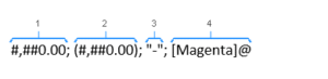
1. Structure Of A Custom Format
A custom format can have up to four sections, separated by semicolons:
- Syntax: Positive;Negative;Zero;Text
- Positive: Format for positive numbers.
- Negative: Format for negative numbers (optional).
- Zero: Format for zero values (optional).
- Text: Format for text entries (optional).
- Example: #,##0;[Red]-#,##0;0;”Text”@
- Positive: 1,234
- Negative: -1,234 in red
- Zero: 0
- Text: Text followed by input (e.g., Text Hello for “Hello”).
- If fewer sections are specified, Excel applies defaults (e.g., #,##0;-#,##0 covers positive and negative, with zeros and text using standard formats). It is one of the crucial custom number formatting features in Excel to look forward to.
Source(Ablebits.com)
2. Key Format Codes
Excel uses specific symbols to build custom formats:
- Numbers:
- 0: Shows a digit, including insignificant zeros (e.g., 00 shows 05 for 5).
- #: Shows significant digits only (e.g., ## shows 5 for 5).
- ?: Adds spaces for alignment (e.g., 0.?? aligns 1.2 and 1.23).
- .: Decimal point (e.g., 0.00 shows 123.45).
- ,: Thousands separator (e.g., #,##0 shows 1,234).
- %: Percentage (e.g., 0% shows 50% for 0.5).
- /: Fractions (e.g., # ?/? shows 3 1/2 for 3.5).
- Currency/Text:
- $, €, etc.: Adds symbols (e.g., $#,##0 shows $1,234).
- “text”: Adds custom text (e.g., 0 “kg” shows 5 kg).
- @: Represents text input (e.g., “Data: “@ shows Data: ABC).
- Dates/Times:
- d, dd: Day without/with leading zero (e.g., d shows 2, dd shows 02 for August 2, 2025).
- mmm, mmmm: Abbreviated/full month (e.g., mmm shows Aug, mmmm shows August).
- yy, yyyy: Two/four-digit year (e.g., yyyy shows 2025).
- h, hh: Hour without/with leading zero (e.g., hh shows 12 for 12:46 PM).
- mm: Minutes or months, depending on context (e.g., hh:mm shows 12:46).
- AM/PM: 12-hour time format (e.g., hh:mm AM/PM shows 12:46 PM).
- Colors/Conditions:
- [Color]: Applies colors (e.g., [Red] for negative numbers; colors include Black, Blue, Cyan, Green, Magenta, Red, White, Yellow).
- [Condition]: Formats based on value (e.g., [>1000]#,##0;”Small” shows 1,234 for >1000, Small for ≤1000).
Source(Ablebits.com)
3. How Excel Applies Formats
Parsing the Code: Excel reads the format code and applies it to the cell’s value. For example, a value of 1234.567 with format #,##0.00 displays as 1,234.57.
Value Preservation: The actual cell value remains unchanged (e.g., 1234.567 is still used in calculations, even if displayed as $1,234.57).
Section Selection: Excel picks the appropriate section based on the value:
- Positive numbers use the first section.
- Negative numbers use the second section (or first if not specified).
- Zero uses the third section (or first if not specified).
- Text uses the fourth section (or displays as entered if not specified).
Locale Impact: Symbols like . or , depend on regional settings (e.g., India uses , for thousands, . for decimals).
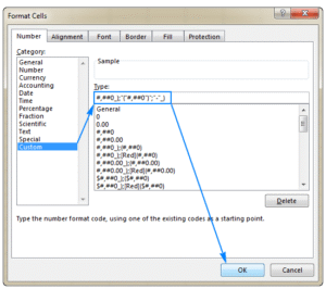
4. Steps To Apply Custom Number Formatting
- Select the cell(s) in Excel.
- Press Ctrl+1 or go to Home > Number Format > More Number Formats.
- In the Format Cells dialog, select Custom.
- Enter the format code in the Type box (e.g., dd-mmm-yyyy for 02-Aug-2025).
- Click OK to apply.
5. Examples In Context
- Currency: $#,##0.00;($#,##0.00) → 1234.56 displays $1,234.56, -1234.56 displays ($1,234.56).
- Date: dd-mmm-yyyy → 44776 (Excel’s date serial for August 2, 2025) displays 02-Aug-2025.
- Time: hh:mm AM/PM → 0.531944 (Excel’s time fraction for 12:46 PM) displays 12:46 PM.
- Units: 0.0 “kg” → 5 displays 5.0 kg.
- Phone Number: (###) ###-#### → 1234567890 displays (123) 456-7890.
- Conditional: [>1000]#,##0;”Small” → 1234 displays 1,234, 500 displays Small.
6. Mechanics Behind Scenes
- Excel’s Value Storage: Numbers are stored as raw values (e.g., 1234.567), dates as serial numbers (e.g., 44776 for August 2, 2025), and times as fractions of a day (e.g., 0.531944 for 12:46 PM).
- Display Layer: Custom formats act as a “mask” that Excel applies to the raw value for display purposes.
- Calculation Integrity: Formulas use the raw value, not the formatted display (e.g., 5.0 kg is treated as 5 in calculations).
- Error Handling: If a format is invalid, Excel may display #### or unexpected results, so testing is key.
7. Limitations
- Display Only: Formats don’t change the cell’s value, so they can’t be used to manipulate data directly.
- Complexity: Complex formats (e.g., multiple conditions) may require careful design.
- Regional Settings: Formats must align with your system’s locale (e.g., , vs . for decimals in India vs. other regions).
How To Apply Custom Number Formatting
Applying custom number formatting in Excel allows you to customize how numbers, dates, times, or text appear in cells without changing their actual values. Below is a step-by-step guide to applying custom number formats, tailored to the current context.
1. Select the Cells
- Highlight the cell or range of cells you want to format.
- Example: Select cells with numbers (e.g., 1234.56), dates (e.g., 44776 for August 2, 2025), times (e.g., 0.6 for 2:24 PM), or text.
2. Open the Format Cells Dialog
- Method 1: Press Ctrl+1 (or Cmd+1 on Mac) to open the Format Cells dialog.
- Method 2:
- Go to the Home tab on the Excel ribbon.
- In the Number group, click the Number Format dropdown (typically shows “General” or another format).
- Select More Number Formats at the bottom.
- Method 3: Right-click the selected cells and choose Format Cells from the context menu.
3. Select The Custom Category
- In the Format Cells dialog, navigate to the Number tab (if not already selected).
- In the Category list on the left, click Custom.
4. Enter The Custom Format Code
- In the Type box, enter the custom format code to define the display.
- Examples (relevant to August 2, 2025, 2:24 PM IST):
- Currency: $#,##0.00;($#,##0.00) → Displays 1234.56 as $1,234.56, -1234.56 as ($1,234.56).
- Date: dd-mmm-yyyy → Displays 44776 as 02-Aug-2025.
- Time: hh:mm AM/PM → Displays 0.6 as 02:24 PM.
- Units: 0.0 “kg” → Displays 5 as 5.0 kg.
- Phone Number: (###) ###-#### → Displays 1234567890 as (123) 456-7890.
- Conditional: [>1000]#,##0;”Small” → Displays 1234 as 1,234, 500 as Small.
- Examples (relevant to August 2, 2025, 2:24 PM IST):
- Check the Sample box in the dialog to preview how the format affects the selected cell’s value.
5. Apply The Format
- Click OK to apply the custom format to the selected cells.
- The cells will now display according to the format code, while the underlying values remain unchanged for calculations.
6. Test And Adjust
- Verify the display in the selected cells. For example:
- A cell with 44776 formatted as dd-mmm-yyyy should show 02-Aug-2025.
- A cell with 0.6 formatted as hh:mm AM/PM should show 02:24 PM.
- If the result is incorrect (e.g., shows #### or unexpected output), reopen the Format Cells dialog and adjust the code.
Benefits Of Using Custom Number Formats
Custom number formatting in Excel allows you to tailor how numbers, dates, times, and text are displayed without altering their underlying values. This provides several benefits, especially in contexts like financial reporting, data presentation, or managing specific formats relevant to August 2, 2025, 2:39 PM IST. Below are the key benefits of using custom number formats:
1. Enhanced Readability And Clarity
- Benefit: Makes data easier to understand by adding context, units, or consistent formatting.
- Examples:
- 0.0 “kg” displays 5 as 5.0 kg, clearly indicating weight.
- #,##0 shows 1234 as 1,234, improving readability for large numbers.
- dd-mmm-yyyy displays 44776 as 02-Aug-2025, making dates intuitive.
- Use Case: Financial reports, inventory lists, or project timelines where clear presentation reduces misinterpretation.
2. Preserves Data Integrity
- Benefit: Changes only the display, not the actual cell value, ensuring calculations remain accurate.
- Example: A cell with 5 formatted as 5.0 kg is still treated as 5 in formulas, avoiding errors in computations.
- Use Case: Scientific data or financial models where underlying values must remain precise.
3. Customized Presentation For Specific Needs
- Benefit: Allows tailored formats for specialized data like phone numbers, IDs, or regional preferences.
- Examples:
- (###) ###-#### formats 1234567890 as (123) 456-7890 for phone numbers.
- 000-00-0000 displays 123456789 as 123-45-6789 for Social Security Numbers.
- #,##0.00 “INR” shows 1234.56 as 1,234.56 INR, aligning with Indian currency formatting.
- Use Case: Customer databases, HR records, or region-specific reports (e.g., India’s date format dd/mm/yyyy).
4. Conditional Formatting For Visual Insights
- Benefit: Enables different displays based on value (positive, negative, zero, or thresholds), highlighting key trends or issues.
- Examples:
- #,##0;[Red]-#,##0;0 shows negative numbers in red (e.g., -1234 as -1,234 in red), drawing attention to losses.
- [>1000]#,##0;”Small” displays 1234 as 1,234 and 500 as Small for quick categorization.
- Use Case: Financial dashboards, performance tracking, or sales reports.
5. Consistent Date And Time Formatting
- Benefit: Customizes date and time displays for clarity and alignment with specific requirements, such as the current context (August 2, 2025, 2:39 PM IST).
- Examples:
- dd-mmm-yyyy shows 44776 as 02-Aug-2025.
- hh:mm AM/PM displays 0.610417 as 02:39 PM.
- dd/mm/yy hh:mm combines to 02/08/25 14:39 for compact logs.
- Use Case: Event schedules, time tracking, or project management reports.
6. Hides Or Customizes Zero Values
- Benefit: Improves report cleanliness by hiding or replacing zero values with custom text.
- Examples:
- #,##0;-#,##0;;@ hides zero values, showing only non-zero numbers or text.
- #,##0;-#,##0;”Zero” displays Zero for 0, making it explicit.
- Use Case: Summary tables or dashboards where zeros are irrelevant or distracting.
Diablo
7. Saves Time And Simplifies Data Entry
- Benefit: Automatically formats data as it’s entered, reducing manual adjustments.
- Example: 00000 ensures a 5-digit ZIP code (e.g., 543 becomes 00543), eliminating the need to type leading zeros.
- Use Case: Data entry forms, order processing, or customer records.
Where Can You Find The Number Formats?
In Excel, number formats, including custom number formats, can be found and applied through specific menus and dialogs. Below is a guide on where to locate number formats, tailored to the context of August 2, 2025, 3:36 PM IST.
1. Home Tab on the Ribbon
- Location:
- Go to the Home tab in the Excel ribbon (at the top of the Excel window).
- In the Number group, locate the Number Format dropdown menu (it typically displays “General” or the current format, like “Number” or “Currency”).
- What You’ll Find:
- Predefined formats such as General, Number, Currency, Accounting, Date, Time, Percentage, Fraction, Scientific, Text, and more.
- At the bottom of the dropdown, select More Number Formats to access the full list, including the Custom category for custom number formats.
- Use Case: Quick access to common formats or to start creating a custom format.
2. Format Cells Dialog
- How to Access:
- Method 1: Select the cell(s), then press Ctrl+1 (or Cmd+1 on Mac) to open the Format Cells dialog.
- Process 2: Right-click the selected cell(s), then choose Format Cells from the context menu.
- Method 3: From the Home tab, click the Number Format dropdown and select More Number Formats.
- What You’ll Find:
- In the Format Cells dialog, go to the Number tab.
- The Category list on the left includes:
- General: Default, no specific formatting.
- Number: For general numbers with decimals and thousands separators.
- Currency: For monetary values (e.g., $1,234.56).
- Accounting: Aligned currency format.
- Date: Predefined date formats (e.g., 02-Aug-2025).
- Time: Predefined time formats (e.g., 15:36 for 3:36 PM).
- Percentage, Fraction, Scientific, Text, Special (e.g., ZIP codes, phone numbers).
- Custom: Allows you to create or edit custom number formats using codes (e.g., dd-mmm-yyyy for 02-Aug-2025 or hh:mm AM/PM for 03:36 PM).
- Use Case: Detailed control over formatting, especially for custom formats like 0.0 “kg” or (###) ###-####.
3. Excel Options (For Default Settings)
- Location:
- Go to File > Options (or Excel Options on Mac).
- Navigate to the Advanced section or search for “number formats.”
- What You’ll Find:
- Options to adjust default number formats based on regional settings (e.g., thousands separator as , in India).
- Not a primary place for applying formats but useful for setting default behaviors.
- Use Case: Adjusting global settings for consistent number formatting across workbooks.
4. Conditional Formatting (For Number-Based Rules)
- Location:
- Go to the Home tab > Conditional Formatting > New Rule.
- Select Format only cells that contain or other rule types.
- Click Format and go to the Number tab to apply number formats conditionally.
- What You’ll Find:
- You can apply number formats (including custom ones) based on cell values (e.g., [Red][<-1000]-#,##0 for negative values below -1000).
- Use Case: Applying number formats dynamically based on data conditions.
5. VBA or Macros (Advanced)
- Location:
- Press Alt+F11 to open the VBA Editor.
- Use VBA code to apply number formats programmatically (e.g., Range(“A1”).NumberFormat = “dd-mmm-yyyy”).
- What You’ll Find:
- Access to the same format codes as in the Custom category of the Format Cells dialog.
- Use Case: Automating number format application for large datasets or repetitive tasks.
Problems & Possible Solutions
Custom number formatting in Excel is powerful for tailoring how numbers, dates, times, and text are displayed, but it can come with challenges.
1. Problem: Format Displays #### Instead of the Expected Output
- Cause: The cell is too narrow to display the formatted value, or the format code is invalid.
- Solution:
- Widen the Column: Double-click the column boundary in the header or manually adjust the column width to fit the formatted content.
- Check the Format Code: Ensure the code is correct. For example, dd-mmm-yyyy displays 02-Aug-2025 for 44776, but an incorrect code like dd-mmm-yyy may cause issues.
- Verify Cell Content: Ensure the cell contains a valid number or date. For instance, text like “abc” won’t format as a date.
- Example: If 44776 shows #### with dd-mmm-yyyy, widen the column or confirm the cell value is a valid date serial number.
2. Problem: Format Doesn’t Apply as Expected
- Cause: The cell’s underlying value doesn’t match the format type (e.g., applying a date format to a number or text).
- Solution:
- Check Data Type: Ensure the cell value aligns with the format. For example, 44776 is a date serial for August 2, 2025, and works with dd-mmm-yyyy, but a text value like “August” won’t.
- Convert Data: Use Text to Columns (under Data tab) or formulas like =VALUE(cell) to convert text to numbers/dates.
- Use General Format First: Set the cell to General format to inspect the raw value, then apply the custom format.
- Example: For a time like 3:46 PM (0.615972), use hh:mm AM/PM to display 03:46 PM. If it’s text, convert it first.
3. Problem: Regional Settings Cause Unexpected Results
- Cause: Format codes may not work as expected due to locale differences (e.g., India uses , for thousands, . for decimals).
- Solution:
- Match Locale: Use symbols consistent with your system’s regional settings. For India, #,##0.00 displays 1,234.56, but in some regions, #.##0,00 is needed.
- Check Regional Settings: Go to File > Options > Advanced and verify decimal/thousands separators.
- Test Locally: For Indian formats, use dd/mm/yyyy for 02/08/2025 or #,##0 “INR” for 1,234 INR.
- Example: If $#,##0.00 shows unexpected results, switch to #,##0.00 “INR” for India.
4. Problem: Negative Numbers Don’t Display as Expected
- Cause: The negative number format section is missing or incorrectly defined in the custom format.
- Solution:
- Define Negative Format: Use a semicolon to specify negative formatting. For example, #,##0;[Red]-#,##0 shows 1,234 for positive and -1,234 in red for negative.
- Add Parentheses: Use #,##0;(#,##0) for 1,234 and (1,234) for negative values, common in financial reports.
- Example: If -1234 shows as 1234, use $#,##0.00;($#,##0.00) to display ($1,234.00).
5. Problem: Zero Values Are Not Hidden or Display Incorrectly
- Cause: The zero section in the format code is missing or not set to suppress zeros.
- Solution:
- Hide Zeros: Use an empty third section (e.g., #,##0;-#,##0;;@) to hide zero values.
- Custom Zero Display: Use #,##0;-#,##0;”Zero”;@ to show Zero for 0.
- Worksheet-Wide Zero Suppression: Go to File > Options > Advanced and uncheck Show a zero in cells that have zero value (affects entire workbook).
- Example: To hide zeros in a sales report, use #,##0;-#,##0;;@ so 0 displays as blank.
6. Problem: Custom Text or Units Don’t Appear
- Cause: Incorrect syntax for adding text or units, or the cell value isn’t compatible.
- Solution:
- Use Quotes for Text: Enclose text in quotes, e.g., 0.0 “kg” displays 5 as 5.0 kg.
- Check for Text Values: If applying text formats (e.g., “Text: “@), ensure the cell contains text, not numbers.
- Escape Special Characters: Use a backslash (e.g., 0\% to show 5% for 5).
- Example: For 5 to show as 5.0 kg, use 0.0 “kg”, not 0.0 kg.
7. Problem: Date or Time Formats Show Incorrectly
- Cause: The cell value isn’t a valid date/time serial number, or the format code is wrong.
- Solution:
- Verify Date/Time Value: Dates are stored as serial numbers (e.g., 44776 for August 2, 2025), and times as fractions (e.g., 0.615972 for 3:46 PM).
- Use Correct Codes: For dates, use dd-mmm-yyyy (displays 02-Aug-2025); for times, use hh:mm AM/PM (displays 03:46 PM).
- Convert Text to Date/Time: Use Date or Time functions, or Text to Columns to convert text like “08/02/2025” to a serial number.
- Example: If 44776 shows as 44776 instead of 02-Aug-2025, apply dd-mmm-yyyy.
8. Problem: Conditional Formats Don’t Work
- Cause: Conditional logic in the format code (e.g., [>1000]) is incorrect or not supported for all sections.
- Solution:
- Use Correct Syntax: Ensure conditions like [>1000]#,##0;”Small” are properly formatted.
- Limit Conditions: Conditions work in the positive/negative sections (e.g., [>1000]#,##0;[<=1000]”Small”), but complex logic may require Conditional Formatting rules instead.
- Test Ranges: Verify the condition covers the data range (e.g., [>1000] for values >1000).
- Example: To show 1,234 for >1000 and Small for ≤1000, use [>1000]#,##0;”Small”.
What Are The Common Shortcuts For Number Formats?
Excel offers some of the keyboard shortcuts in order to meet common formats. Some of the shortcut keys are as follows:-
| Format | Shortcut Keys |
|---|---|
| General Format | Ctrl Shift ~ |
| Currency Format | Ctrl Shift $ |
| Date Format | Ctrl Shift # |
| Percentage Format | Ctrl Shift % |
| Custom Format | Ctrl +1 |
| Scientific Format | Ctrl Shift ^ |
| Time Format | Ctrl Shift @ |
Different Ways To Format Numbers In Excel
Formatting numbers in Excel allows you to customize how numerical data is displayed without altering the underlying values. Below are the primary ways to format numbers in Excel, including built-in formats, custom formats, and other techniques. Each method is explained with its purpose and steps to apply it.
1. General
Default format, displays numbers as entered (e.g., 1234.567 → 1234.567). In this format, it will show the numbers in the order you type them. It may happen that the cell is not wide enough then to display all the complete places you must round the number to a smaller decimal. In most of the cases, all these formats make use of scientific notations.
2. Number
Adds decimal places and optional thousands separators (e.g., 1234.567 with 2 decimals → 1,234.57). This format will help you to display different kinds of numbers such as decimal, large numbers, and negative numbers. In each cell and row you can select the numbers in the decimal places that you want.
3. Currency
Includes a currency symbol and 2 decimal places (e.g., 1234.567 → $1,234.57). However, you can make use of the currency formats to organize and display all the monetary values. Whenever you do it you can make use of default symbols as well as currency. It is easier for you to use specific symbols depending on the currency you make use of.
4. Accounting
Aligns currency symbols and decimals, shows zeros as dashes (e.g., 0 → $ -). You can easily decide on the decimals and symbol points that you want to group. Almost like the dollar symbols with any other numbers that have two decimal places.
5. Date & Time
The date number format shows the time and date within the cell. There are numerous ways to employ or use display information. You can share your views in this regard while you adjust the date and time.
FAQ(Frequently Asked Questions)
1. How do You create a custom format to show negative numbers in red and parentheses?
Use this format code:
#,##0;[Red]($#,##0)
- #,##0 → Positive numbers with thousand separators
- [Red]($#,##0) → Negative numbers in red and parentheses Example: 1234 → 1,234 | -5678 → (5,678) in red
Tip: You can also add conditions like [>1000]$#,##0.00;[Red][<=-1000]($#,##0.00);0 for large values.
2. How can You display phone numbers as (123) 456-7890 using custom formatting?
Enter this format:
(###) ###-####
- Works only if the number is entered as 10 digits (e.g., 1234567890)
- Excel treats it as text-like display but keeps the numeric value
Alternative for flexibility: +1 (###) ###-#### → +1 (123) 456-7890
3. How do You show text with numbers, like “Total: $1,234”?
Use:
“Total: “$#,##0
- The text in quotes appears literally
- $#,##0 formats the number
Pro trick: Combine with conditions:
“Profit: “$#,##0;”Loss: “($#,##0) → Shows “Profit” or “Loss” based on sign.
4. How do You hide zero values but still keep the cell functional?
Use this format:
#,##0;-#,##0;;
- First section: positive
- Second: negative
- Third: zero (left blank)
- Fourth: text (optional)
Result: 0 displays as blank, but formulas still read the value.
Caution: Don’t confuse with 0;-0;;@ — that hides zeros and treats them as text.
5. How do You add conditional formatting with colors AND custom number formats?
Custom number formats support 4 conditions using [Color] and brackets:
[Green]$#,##0;[Red]-$#,##0;[Blue]0;[Black]”N/A”
- Green for positive
- Red for negative
- Blue for zero
- Black text “N/A” for text entries
Advanced example (threshold-based):
[>=1000]$#,##0.00;[>=0]$#,##0.00;[Red]-$#,##0.00
→ Large positives in default color, small positives too, negatives in red.
Final Takeaway
Hence, these are some of the crucial factors of Custom number formatting in Excel that you must know from your end. Ensure that you follow the correct methods to use these functions of excel to enhance your productivity.
You can share your views and opinions in our comment box. This will help us to know your take on this matter. Ensure that you follow the correct methodologies to optimize the perfect method for custom number formatting.